“NN4SysBench is a benchmark suite for neural network verification, incorporating applications from the domain of neural network for computer systems (NN4Sys). This suite includes verification benchmark for learned index, learned bloom filter, learned cardinality, learned Internet congestion control, learned adaptive bitrate, learned distributed system scheduler, which are six tasks that apply neural networks to solve traditional tasks for systems.
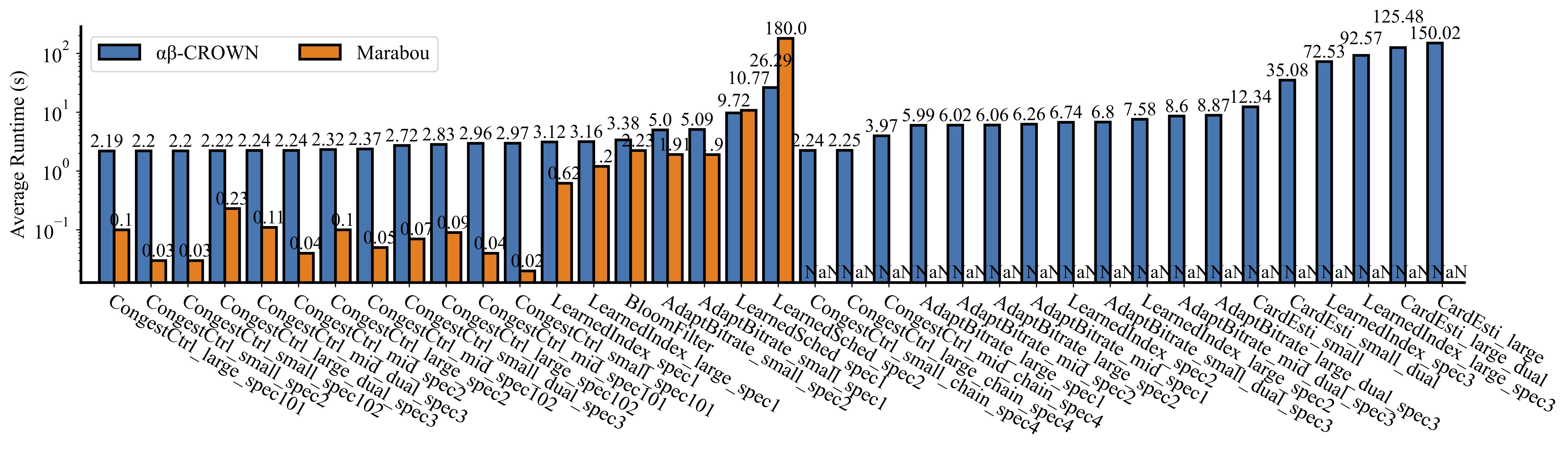
Results of different verifiers (Hover to zoom in for a closer look):
Applications
Learned Index
A database index is a data structure that improves data retrieval by linking database keys to their storage positions. Learned indexes replace traditional structures like B-Trees with ML models that predict storage locations based on database keys. For more information, check out the paper.
Neural Network
Original Paper
The original paper introduces Recursive Model Index (RMI), a framework that leverages a set of machine learning models to construct a hierarchical graph. The final implementation opts for linear models instead of neural networks to enhance execution performance. The initial naive design employs a two-layer fully connected neural network with 32 neurons. However, training a neural network to accurately model the database proves to be challenging.
Our Implementation
We use neural networks to learn database index. We have two sizes of neural networks:
1. LINN (Lightweight Neural Network):
- Width: 128 neurons per hidden layer.
- Depth: 4 layers (3 fully connected layers followed by ReLU activations and 1 output layer).
2. DeepLINN (Deep Lightweight Neural Network):
- Width: 128 neurons per hidden layer.
- Depth: 6 layers (5 fully connected layers with ReLU activations).
We face the same challenge as the original paper. We train the models via a
training-verification loop.
Specification
All predicted data locations are error-bounded.
Performance of the Verifier
| Verifier | Type | Safe | Unsafe | Time | Timeout |
|---|---|---|---|---|---|
| abcrown | lindex_0 | 10 | 0 | 3.12916079 | 0 |
| marabou | lindex_0 | 10 | 0 | 0.621874303 | 0 |
| abcrown | lindex_1 | 10 | 0 | 6.74826283 | 0 |
| abcrown | lindex_2 | 10 | 0 | 72.5362575 | 0 |
| abcrown | lindex_deep_0 | 10 | 0 | 3.16443444 | 0 |
| marabou | lindex_deep_0 | 10 | 0 | 1.201228401 | 0 |
| abcrown | lindex_deep_1 | 10 | 0 | 7.58243066 | 0 |
| abcrown | lindex_deep_2 | 7 | 0 | 92.5729578 | 3 |
Learned Bloom Filter
A bloom filter is a probabilistic data structure that has been widely used in many computer systems. Bloom filters test whether an element (for example, a string) is in a pre-defined set. Bloom filters allow false positives: it may return true for an element that is not in the set. The inputs are being-tested elements, and the outputs are booleans, whether the elements are in the set. For more information, check out the paper.
Neural Network
Original Paper
The original paper introduces Learned Bloom Filter, a compact replacement for traditional Bloom filters that leverages a binary classifier to distinguish between keys and non-keys. The initial implementation uses a recurrent neural network (GRU) with 16 hidden units and a 32-dimensional character embedding to process string inputs. While the model achieves high classification accuracy, it cannot guarantee zero false negatives. To address this limitation, the final design incorporates an auxiliary Bloom filter to catch any missed keys, thereby ensuring correctness while reducing overall memory consumption.
Our Implementation
We use neural networks to learn Bloom filters. Our architecture is as follows:
- Width: 256 neurons per hidden layer.
- Depth: 4 layers (3 fully connected layers followed by ReLU activations, and 1 final output layer).
- Output: A sigmoid activation is applied to produce a probability indicating key membership.
This model takes a 2-dimensional input and predicts whether a given key belongs to the target set.
Specification
The false positive and false negative rates are bounded.
Performance of the Verifier
| Verifier | Type | Safe | Unsafe | Time | Timeout |
|---|---|---|---|---|---|
| abcrown | bloom_filter | 10 | 0 | 3.38892075 | 0 |
| marabou | bloom_filter | 10 | 0 | 2.23303003 | 0 |
Learned Cardinality
database cardinality estimation predicts the number of rows returned by a database query (i.e., a SQL statement), which will then influence the query optimization plans. Traditional cardinality estimation relies on heuristics and domain knowledge; whereas, the learned cardinalities learn from the trace data. The inputs of learned cardinalities are SQL queries, and the outputs are estimated number of returned rows. For more information, check out the paper.
Neural Network
Original Paper
The paper proposes MSCN (Multi-Set Convolutional Network) for cardinality estimation. It uses three two-layer neural networks to process different parts of a SQL query: tables, joins, and predicates. Each part goes through a shared MLP:
- Linear → ReLU → Linear → ReLU
The outputs from each set are averaged, then merged and passed into a final output network:
- Linear → ReLU → Linear → Sigmoid
This design helps the model handle different query structures and capture complex data patterns. It works better than traditional sampling methods, especially when no qualifying samples exist. The model is small (about 2–3MB) and trained with q-error as the loss.
Our Implementation
We use neural networks to learn database query patterns. We implemented four variations of our SetConv architecture:
1. MSCN-128d:
- Width: 128 neurons per hidden layer
- Depth: 2 hidden layers in each feature path + 2 layers for combined features
- Training: 10,000 queries, 10 epochs, batch size of 1024, learning rate of 0.01
2. MSCN-128d-dual:
- Width: 128 neurons per hidden layer
- Depth: 2 hidden layers in each feature path + 2 layers for combined features
- Processing: Dual parallel paths with subtraction operation for final output
- Training: 10,000 queries, 10 epochs, batch size of 1024, learning rate of 0.01
3. MSCN-2048d:
- Width: 2048 neurons per hidden layer
- Depth: 2 hidden layers in each feature path + 2 layers for combined features
- Training: 10,000 queries, 10 epochs, batch size of 1024, learning rate of 0.01
4. MSCN-2048d-dual:
- Width: 2048 neurons per hidden layer
- Depth: 2 hidden layers in each feature path + 2 layers for combined features
- Processing: Dual parallel paths with subtraction operation for final output
- Training: 10,000 queries, 10 epochs, batch size of 1024, learning rate of 0.01
Our model processes input features of varying dimensions: sample features (based on table vectors), predicate features (combining column vectors, operation vectors, and values), and join features. Each feature type is processed through its own two-layer MLP with ReLU activations before being combined. We face the same challenges as the original paper and train our models via a training-verification loop to ensure model accuracy and generalization.
Specification
The predicted cardinalities are close to the ground-truth cardinalities from the database. A larger-ranged query returns larger cardinality.
Performance of the Verifier
| Verifier | Type | Safe | Unsafe | Time | Timeout |
|---|---|---|---|---|---|
| abcrown | mscn_128d | 10 | 0 | 12.3426136 | 0 |
| abcrown | mscn_128d_dual | 10 | 0 | 35.0842626 | 0 |
| abcrown | mscn_2048d | 3 | 0 | 150.021686 | 7 |
| abcrown | mscn_2048d_dual | 6 | 0 | 125.487949 | 4 |
Learned Internet Congestion Control
Congestion control protocols are to ensure efficient data transmission and prevent packet congestion in a network. Learned congestion control studies the patterns of congestion and non-congestion conditions, takes network conditions as input, and decides sending rates in the near future. For more information, check out the paper.
Neural Network
Original Paper
The neural network (NN) described in the Aurora paper is a small, fully connected neural network with the following architecture:
- Two hidden layers consisting of 32 and 16 neurons, respectively.
- The activation function used is the hyperbolic tangent (tanh).
Input:
The input is a tensor with K history, each time step contains the following features:
1. Latency gradient: latency/time
2. Latency ratio: Current MI's mean latency / observed mean latency of any MI
3. Sending ratio: packets sent / packets acknowledged by the receiver
All the input tensors are flattened into a 1D tensor.
Output:
1. Change of Sending rate: positive value means increase, negative value means decrease
Our Implementation
In our benchmark, considering the limitation of current verifiers, we implement a compatible version of this neural network architecture. Implementation can be found in our repository.
To create different difficulty of the verification, we provide 3 different sizes of the model:
- Small model:
2 hidden layers of 16 → 8 neurons, tanh nonlinearity.
- Mid model (same as original paper):
2 hidden layers of 32 → 16 neurons, tanh nonlinearity.
- Big model:
2 hidden layers of 32 → 16 neurons, tanh nonlinearity.
Specification
CongestCtrl_spec101/102: When observing good (bad) networking conditions, the sender does not decrease (increase) packet sending rates.
CongestCtrl_spec2: When observing better networking conditions, the sender increases packet sending rates by either the same or a larger amount.
CongestCtrl_spec3: When the networking condition changes from bad to good, the sender eventually increases packet sending rates.
Performance of the Verifier
| Verifier | Type | Safe | Unsafe | Time | Timeout |
|---|---|---|---|---|---|
| abcrown | aurora_big_101 | 0 | 10 | 2.19588738 | 0 |
| marabou | aurora_big_101 | 0 | 10 | 0.102064294 | 0 |
| abcrown | aurora_big_102 | 6 | 4 | 2.838494590 | 0 |
| marabou | aurora_big_102 | 6 | 4 | 0.09996135 | 0 |
| abcrown | aurora_big_2 | 0 | 10 | 2.32072963 | 0 |
| marabou | aurora_big_2 | 0 | 10 | 0.102983946 | 0 |
| abcrown | aurora_big_3 | 0 | 10 | 2.22639322 | 0 |
| marabou | aurora_big_3 | 0 | 10 | 0.23421416 | 0 |
| abcrown | aurora_big_4 | 0 | 10 | 2.25798789 | 0 |
| abcrown | aurora_mid_101 | 10 | 0 | 2.96464823 | 0 |
| marabou | aurora_mid_101 | 10 | 0 | 0.042553444 | 0 |
| abcrown | aurora_mid_102 | 0 | 10 | 2.37557136 | 0 |
| marabou | aurora_mid_102 | 0 | 10 | 0.053586597 | 0 |
| abcrown | aurora_mid_2 | 0 | 10 | 2.24732022 | 0 |
| marabou | aurora_mid_2 | 0 | 10 | 0.049091978 | 0 |
| abcrown | aurora_mid_3 | 0 | 10 | 2.24376578 | 0 |
| marabou | aurora_mid_3 | 0 | 10 | 0.113317223 | 0 |
| abcrown | aurora_mid_4 | 10 | 0 | 3.97856824 | 0 |
Learned Adaptive Bitrate
In video streaming, adaptive bitrate algorithms are used on client-side video players to decide the resolution (e.g., 720P) to download for the next video chunk. Learned adaptive bitrate uses neural networks to select future video chunks based on observations collected by client video players. For more information, check out the paper.
Neural Network
Original Paper
The neural network (NN) in the Pensieve paper is a deep feedforward neural network used for adaptive bitrate control in video streaming. It takes multiple input features related to video playback, network conditions, and device performance. These inputs are processed through several hidden layers to predict the optimal video bitrate that maximizes quality while minimizing interruptions like buffering.
Input:
The input is a tensor with N history time steps, each time step contains the following features:- Last chunk bitrate: bitrate/max bitrate, ex: 360P/1080P
- Past chunk download time
- Next chunk sizes
- Current buffer size
- Number of chunks left: eg: 43/48
- Past chunk throughput:
Output:
- optimal video bitrate
Our Implementation
In our benchmark, considering the limitation of current verifiers, we implement a compatible version of this neural network architecture. We implement 2 versions, benchmark version and a version for marabou the verifier. Implementation can be found in our repository.
Benchmark Version
The model is almost the same as the original paper, except that we remove the softmax and argmax layers, and all the input tensors are flattened into a 1D tensor. The input and output can be referred to in the Original Paper section.
To create different difficulty of the verification, we provide 3 different sizes of the model:
Small model:
- First Layer: 4 parallel fully connected layers, each containing 128 neurons
- Second Layer: A fully connected (linear) layer with 128 neurons
- Output Layer: Fully connected (linear) layer with 6 neurons
Mid model (same as original paper):
- First Layer: 3 parallel fully connected layers, each containing 128 neurons, and a 1D convolution layer with 128 filters and kernel size 4. These 4 layers take the input features in parallel.
- Second Layer: A fully connected (linear) layer with 128 neurons
- Output Layer: A fully connected (linear) layer with 6 neurons
Big model:
- First Layer: 3 parallel fully connected layers, each containing 128 neurons, and a 1D convolution layer with 128 filters and kernel size 4. These 4 layers are parallel.
- Second Layer: A fully connected (linear) layer with 256 neurons
- Output Layer: Fully connected (linear) layer with 6 neurons
Marabou Version
Main difference:
- Use torch.split() to split the input tensor into 2 parts.
Specification
AdaptiveBitrate_spec1/2: When facing good (bad) downloading conditions, the video streaming system should not
pick the worst (best) video resolution.
AdaptiveBitrate_spec3: Better downloading conditions implies better resolutions
Performance of the Verifier
| Verifier | Type | Safe | Unsafe | Time | Timeout |
|---|---|---|---|---|---|
| abcrown | pensieve_big_1 | 10 | 0 | 5.99909349 | 0 |
| abcrown | pensieve_big_2 | 10 | 0 | 6.06507417 | 0 |
| abcrown | pensieve_big_3 | 10 | 0 | 8.87928039 | 0 |
| abcrown | pensieve_mid_1 | 10 | 0 | 6.26007705 | 0 |
| abcrown | pensieve_mid_2 | 10 | 0 | 6.02888779 | 0 |
| abcrown | pensieve_mid_3 | 10 | 0 | 8.6088345 | 0 |
| abcrown | pensieve_small_1 | 10 | 0 | 5.0981046 | 0 |
| marabou | pensieve_small_1 | 10 | 0 | 1.90850646 | 0 |
| abcrown | pensieve_small_2 | 10 | 0 | 5.00802932 | 0 |
| marabou | pensieve_small_2 | 10 | 0 | 1.91794796 | 0 |
| abcrown | pensieve_small_3 | 10 | 0 | 6.80163713 | 0 |
Learned Distributed System Scheduler
The System Scheduler is designed for distributed computing systems like Spark. It manages a cluster of machines running multiple jobs, each with tasks that have dependencies. Using neural networks, a learned scheduler optimizes task scheduling to achieve high-level objectives, such as minimizing job completion time. It takes inputs like the status of jobs, tasks, and the cluster, and outputs the next tasks to run. For more information, check out the paper.
Neural Network
Original Paper
The original neural network architecture consists of three main components:
1. GCN (Graph Convolutional Network)
- Models dependencies between tasks and jobs
- Captures graph structure of task interdependencies
2. GSN (Graph Scheduling Network)
- Builds on the GCN output
- Focuses on scheduling optimization
- Predicts optimal task schedules using graph-structured data
3. FC (Fully Connected) Layers
- Refines representations from GCN and GSN
- Outputs final scheduling decisions
- Determines next tasks to execute
These components work together to enable efficient task scheduling in distributed systems through dynamic, data-driven decisions.
Our Implementation
In our benchmark, considering the limitation of current verifiers, we implement a compatible version of this neural network architecture. We implement 2 versions, benchmark version and a version for marabou the verifier. Implementation can be found in our repository.
We integrate the 3 components into a single neural network. The input is the status of jobs, tasks, and the cluster, and the output is the next tasks to execute.
Benchmark Version
Input:
The input to the model is a tensor that is split into several segments:
All the input tensors are flattened into a 1D tensor.
Shape: [batch_size, Max_Node, 5]
Shape: [batch_size, 1, Max_Node]
Shape: [batch_size, 8, Max_Node, Max_Node]
Shape: [batch_size, 8, Max_Node, 1]
Shape: [batch_size, Max_Node, Max_Node]
Shape: [batch_size, 1, Max_Node]
Shape: [batch_size, Max_Node, Max_Node]Output:
Shape: [1, node_num]
Shape: [1, job_num, total_executor_num]
Marabou Version
Most of the architecture is the same as the benchmark version, with a few key differences such as the use of a different graph convolution layer (GraphLayer_marabou) and learnable parameters for matrices like gcn_mats and gcn_masks.
Specification
LearnedSched_spec1: If job A's input depends on job B's output and job B is not finished, then job A should not be scheduled.
LearnedSched_spec2: A user cannot get their jobs scheduled earlier by requesting more resources for them.
Performance of the Verifier
| Verifier | Type | Safe | Unsafe | Time | Timeout |
|---|---|---|---|---|---|
| abcrown | decima_mid_1 | 10 | 0 | 9.7232395 | 0 |
| marabou | decima_mid_1 | 10 | 0 | 10.77956162 | 0 |
| abcrown | decima_mid_2 | 8 | 1 | 26.29458285 | 1 |
| marabou | decima_mid_2 | 0 | 0 | 180.0 | 10 |